User Guide

GAMA is an AutoML tool which aims to automatically find the right machine learning algorithms to create the best possible data for your model. This page gives an introduction to basic components and concepts of GAMA.

GAMA performs a search over machine learning pipelines. An example of a machine learning pipeline would be to first perform data normalization and then use a nearest neighbor classifier to make a prediction on the normalized data. More formally, a machine learning pipeline is a sequence of one or more components. A component is an algorithm which performs either data transformation or a prediction. This means that components can be preprocessing algorithms such as PCA or standard scaling, or a predictor such as a decision tree or support vector machine. A machine learning pipeline then consists of zero or more preprocessing components followed by a predictor component.

Given some data, GAMA will start a search to try and find the best possible machine learning pipelines for it. After the search, the best model found can be used to make predictions. Alternatively, GAMA can combine several models into an ensemble to take into account more than one model when making predictions. For ease of use, GAMA provides a fit, predict and predict_proba function akin to scikit-learn.

Installation

For regular usage, you can install GAMA with pip:

pip install gama

GAMA features optional dependencies for visualization and development. You can install them with:

pip install gama[OPTIONAL]

where OPTIONAL is one or more (comma separated):

• vis: allows you to use the prototype dash app to visualize optimization traces.

• dev: sets up all required dependencies for development of GAMA.

• doc: sets up all required dependencies for building documentation of GAMA.

To see exactly what dependencies will be installed, see setup.py. If you plan on developing GAMA, cloning the repository and installing locally with test and doc dependencies is advised:

git clone https://github.com/PGijsbers/gama.git
cd gama
pip install -e ".[doc,test]"

This installation will refer to your local GAMA files. Changes to the code directly affect the installed GAMA package without requiring a reinstall.

---

Examples

Classification

from sklearn.datasets import load_breast_cancer
from sklearn.model_selection import train_test_split
from sklearn.metrics import log_loss, accuracy_score
from gama import GamaClassifier

if __name__ == "__main__":
    X, y = load_breast_cancer(return_X_y=True)
    X_train, X_test, y_train, y_test = train_test_split(
        X, y, stratify=y, random_state=0
    )

    automl = GamaClassifier(max_total_time=180, store="nothing", n_jobs=1)
    print("Starting `fit` which will take roughly 3 minutes.")
    automl.fit(X_train, y_train)

    label_predictions = automl.predict(X_test)
    probability_predictions = automl.predict_proba(X_test)

    print("accuracy:", accuracy_score(y_test, label_predictions))
    print("log loss:", log_loss(y_test, probability_predictions))

Should take 3 minutes to run and give the output below (exact performance might differ):

accuracy: 0.951048951048951
log loss: 0.1111237013184977

By default, GamaClassifier will optimize towards log loss.

Regression

from sklearn.datasets import load_boston
from sklearn.model_selection import train_test_split
from sklearn.metrics import mean_squared_error
from gama import GamaRegressor

if __name__ == "__main__":
    X, y = load_boston(return_X_y=True)
    X_train, X_test, y_train, y_test = train_test_split(X, y, random_state=0)

    automl = GamaRegressor(max_total_time=180, store="nothing", n_jobs=1)
    print("Starting `fit` which will take roughly 3 minutes.")
    automl.fit(X_train, y_train)

    predictions = automl.predict(X_test)

    print("MSE:", mean_squared_error(y_test, predictions))

Should take 3 minutes to run and give the output below (exact performance might differ):

MSE: 19.238475470025886

By default, GamaRegressor will optimize towards mean squared error.

Using Files Directly

You can load data directly from csv and ARFF files. For ARFF files, GAMA can utilize extra information given, such as which features are categorical. For csv files GAMA will infer column types, but this might lead to mistakes. In the example below, make sure to replace the file paths to the files to be used. The example script can be run by using e.g. breast_cancer_train.arff and breast_cancer_test.arff. The target should always be specified as the last column, unless the target_column is specified. Make sure you adjust the file path if not executed from the examples directory.

from gama import GamaClassifier

if __name__ == "__main__":
    file_path = "../tests/data/breast_cancer_{}.arff"

    automl = GamaClassifier(max_total_time=180, store="nothing", n_jobs=1)
    print("Starting `fit` which will take roughly 3 minutes.")
    automl.fit_from_file(file_path.format("train"))

    label_predictions = automl.predict_from_file(file_path.format("test"))
    probability_predictions = automl.predict_proba_from_file(file_path.format("test"))

The GamaRegressor also has csv and ARFF support.

The advantage of using an ARFF file over something like a numpy-array or a csv file is that attribute types are specified. When supplying only numpy-arrays (e.g. through fit(X, y)), GAMA can not know if a particular feature is nominal or numeric. This means that GAMA might use a wrong feature transformation for the data (e.g. one-hot encoding on a numeric feature or scaling on a categorical feature). Note that this is not unique to GAMA, but any framework which accepts numeric input without meta-data.

Note

Unfortunately the date and string formats the ARFF file allows is not (fully) supported in GAMA yet, for the latest news, see issue#2.

---

Simple Features

This section features a couple of simple to use features that might be interesting for a wide audience. For more advanced features, see the Advanced Guide.

Command Line Interface

GAMA may also be called from a terminal, but the tool currently supports only part of all Python functionality. In particular it can only load data from .csv or .arff files and AutoML pipeline configuration is not available. The tool will produce a single pickled scikit-learn model (by default named ‘gama_model.pkl’), code export is also available. Please see gama -h for all options.

Code Export

It is possible to have GAMA export the final model definition as a Python file, see gama.Gama.export_script().

---

Dashboard

Note

The GAMA Dashboard is not done. However, it is functional and released to get some early feedback on what users would like to see included. The near future may see a reimplementation, see #97.

GAMA Dashboard is a graphical user interface to start and monitor the AutoML search. It is available when GAMA has been installed with its visualization optional dependencies (pip install gama[vis]). To start GAMA Dashboard call gamadash from the command line.

Home tab

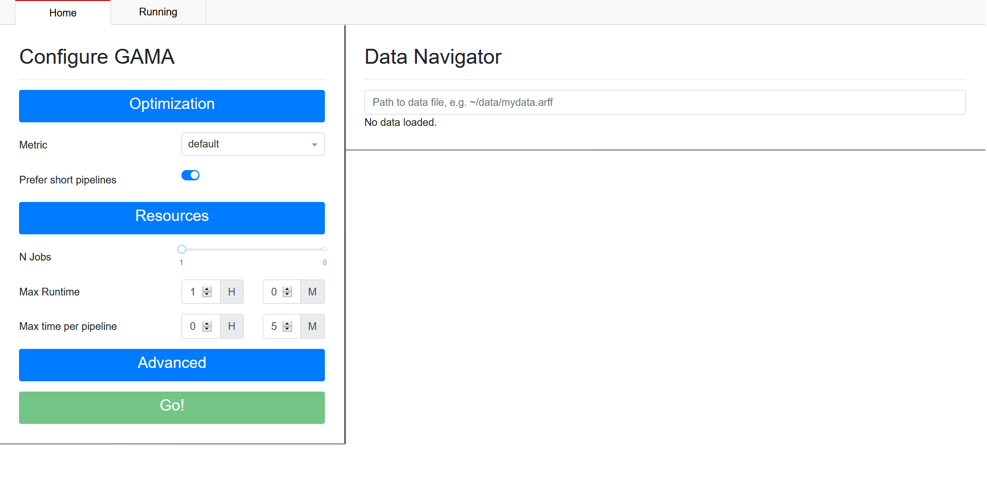
Starting GAMA Dashboard will open a new tab in your webbrowser which will show the GAMA Dashboard Home page:

On the left you can configure GAMA, on the right you can select the dataset you want to perform AutoML on. To provide a dataset, specify the path to the csv or ARFF-file which contains your data. Once the dataset has been set, the Go!-button on the bottom left will be enabled. When you are satisfied with your chosen configuration, press the Go!-button to start GAMA. This will take you to the ‘Running’ tab.

Running tab

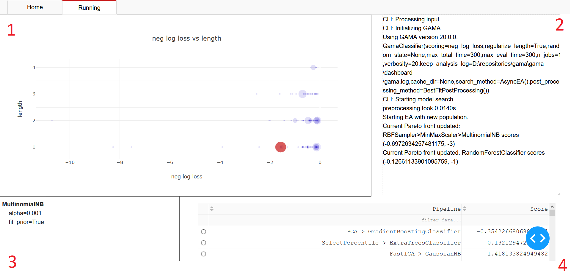
The running tab will look similar to this:

You see four main components on this page:

1. A visualization of search results. In this scatter plot, each scored pipeline is represented by a marker. The larger markers represent the most recent evaluations. Their location is determined by the pipeline’s length (on the y-axis) and score (on the x-axis). You can hover over the markers to get precise scores, and click on the pipeline to select it. A selected pipeline is represented with a large red marker.

2. Output of the search command. This field provides a textual progress report on GAMA’s AutoML process.

3. Full specification of the selected pipeline. This view of the selected pipeline specifies hyperparametersettings for each step in the pipeline.

4. A table of each evaluated pipeline. Similar to the plot (1), here you find all pipelines evaluated during search. It is possible to sort and filter based on performance.

Selecting a pipeline in the table or through the plot will update the other components.

Analysis tab

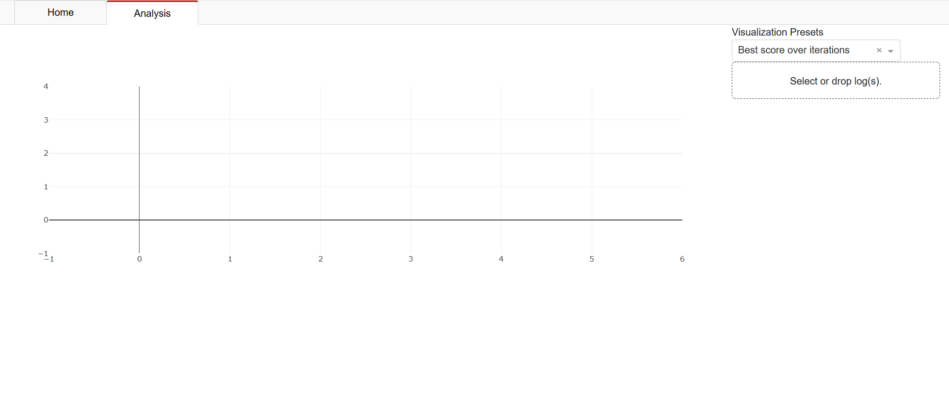
The analysis tab is also available if you did not start a new GAMA run. On this tab, you can visualize search results from logs.

Clicking ‘Select or drop log(s)’ in the top-right corner opens a file explorer which lets you select file(s) to load. Select both the ‘gama.log’ and ‘evaluation.log’ files from your directory together. For example the the logs found here. After loading the files, you can toggle its visualization by clicking the checkbox that appears next to the file name. The first visualization you will see is the best obtained score as a function of the number of evaluated pipelines:

In the top right you will find a dropdown ‘Visualization Presets’ which allow you to see other visualizations. Below you will find a description of each preset.

Visualization presets include:

• #Pipeline by learner A bar chart of the number of times each estimator is used as the final step in a machine learning pipeline.

• #Pipeline by size A bar chart of the distribution of the number of components per evaluated pipeline.

• Best score over time The best score obtained by any individual pipeline at a given point in time.

• Best score over iterations The best score obtained by any individual pipeline at a given iteration.

• Size vs Metric A scatter plot where each pipeline is represented by a marker, gives an impression of the distribution of scores for evaluated pipelines of different lengths.

• Evaluation Times A bar chart plotting the distribution of time required to evaluate pipelines during optimization.

• Evaluations by Rung (ASHA only) A bar chart plotting the number of evaluations at each ASHA rung.

• Time by Rung (ASHA only) A bar chart plotting the combined time used of all evaluations for each ASHA rung.

---

Important Hyperparameters

There are a lot of hyperparameters exposed in GAMA. In this section, you will find some hyperparameters you might want to set even if you otherwise use defaults. For more complete documentation on all hyperparameters, see API documentation.

Optimization

Perhaps the most important hyperparameters are the ones that specify what to optimize for, these are:

scoring: string (default=’neg_log_loss’ for classification and ‘mean_squared_error’ for regression)

Sets the metric to optimize for. Make sure to optimize towards the metric that reflects well what is important to you. Any string that can construct a scikit-learn scorer is accepted, see this page for more information. Valid options include roc_auc, accuracy and neg_log_loss for classification, and neg_mean_squared_error and r2 for regression.

regularize_length: bool (default=True)

If True, in addition to optimizing towards the metric set in scoring, also guide the search towards shorter pipelines. This setting currently has no effect for non-default search methods.

Example:

GamaClassifier(scoring='roc_auc', regularize_length=False)

Resources

n_jobs: int, optional (default=None)

Determines how many processes can be run in parallel during fit. This has the most influence over how many machine learning pipelines can be evaluated. If it is set to -1, all cores are used. If set to None (default), half the cores are used. Changing it to use a set amount of (fewer) cores will decrease the amount of pipelines evaluated, but is needed if you do not want GAMA to use all resources.

max_total_time: int (default=3600)

The maximum time in seconds that GAMA should aim to use to construct a model from the data. By default GAMA uses one hour. For large datasets, more time may be needed to get useful results.

max_eval_time: int (default=300)

The maximum time in seconds that GAMA is allowed to use to evaluate a single machine learning pipeline. The default is set to five minutes. For large datasets, more time may be needed to get useful results.

Example:

GamaClassifier(n_jobs=2, max_total_time=7200, max_eval_time=600)

---

Related Packages

There are many different AutoML packages in Python and other languages. This webpage of the AutoML Benchmark project has an overview of commonly used open source AutoML frameworks. Another nice overview of papers and projects is gathered at this Github repo.

Note

Any comparisons in this section are intended to highlight the main differences, but are by no means exhaustive. If anything is missing that is important to add, please open an issue.

TPOT

TPOT is the package most closely related to GAMA. Like GAMA, it is an AutoML package that is based on genetic programming in Python. Below you will find a list of differences and similarities of the packages.

The evolution algorithm differs. TPOT uses a synchronous form of evolution, whereas GAMA uses asynchronous evolution (by default). The advantage of asynchronous evolution is that in theory it is able to utilize computing resources better. This is due to generation-based evolution waiting for the last individual in the population to be evaluated in each generation, whereas asynchronous evolution does not have any point where all evaluations need to be finished at the same time.

TPOT sports some great user-friendly features such as a less limited command-line interface and DASK integration (which allows the use of a Dask cluster for pipeline evaluations and further optimizations).

GAMA focuses more on extensibility and research friendliness, with the ability to configure your AutoML pipeline (for instance using a different search strategy), an ensembling post-processing step, visualization of the optimization process and support for ARFF files.

auto-sklearn

auto-sklearn is another AutoML package in Python. It uses Bayesian optimization to search for good machine learning pipelines and also features automatic ensemble construction. Auto-sklearn won ChaLearn AutoML challenge 1 and 2.